


The Chi-Square Test of Goodness of Fit is a statistical method used to determine whether a set of observed frequencies significantly differs from expected frequencies derived from a particular theoretical distribution. This non-parametric test is widely applied when dealing with categorical data, helping researchers and analysts assess how well a theoretical model fits real-world data.
When to Use?
Use this test when:
- You have one categorical variable.
- You want to compare observed data with expected frequencies.
- Data must be in counts (frequencies), not percentages or means.
Key Assumptions:
- Data should be categorical.
- Categories are mutually exclusive.
- Expected frequency in each category should be at least 5.
- Observations must be independent.
Formula:
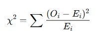
Where:
- Oi = Observed frequency
- Ei = Expected frequency
- The result is compared against a critical value from the Chi-Square distribution table at a given degree of freedom (df = k – 1).
Example research questions:
Are customer preferences for different drink flavours equally distributed?
Do birth rates follow an expected gender ratio?
Do voter preferences match predicted proportions?
Is distribution of blood types in a small sample matches the national average proportions?
Example Scenario:
Do students have an equal preference for four types of extracurricular activities: Sports, Music, Art, and Debate?
Step 1: Define Hypotheses
Null Hypothesis (H₀): Preferences are equally distributed (25% each).
Alternative Hypothesis (H₁): Preferences are not equally distributed.
Step 2: Collect Observed Data
Collect the data extracurricular activities-wise as Observed Frequency
Step 3: Determine Expected Frequencies
Since preferences are expected to be equal:
Expected frequency (E) for each = Total / Number of categories = 100 / 4 = 25
Step 4: Apply the Chi-Square Formula
CHI-SQUARE TEST TABLE
| Activity | Observed (O) | Expected (E) | (O-E) | (O-E)2 | (O-E)2 E |
| Sports | 40 | 25 | 15 | 225 | 9.00 |
| Music | 25 | 25 | 0 | 0 | 0.00 |
| Arts | 20 | 25 | -5 | 25 | 1.00 |
| Debate | 15 | 25 | -10 | 100 | 4.00 |
| Total χ² | 14.00 | ||||
Step 5: Degrees of Freedom (df)
DF = Number of Categories – 1 = 4 – 1 = 3
Step 6: Decision Rule
Critical value of χ² at df = 3, α = 0.05 = 7.815
Since calculated χ² = 14.00 > 7.815, reject the null hypothesis
Final Interpretation
There is a significant difference in students’ preferences across the four activities. The preferences are not equally distributed.
Interpretation Guidelines:
If Chi-Square > critical value, reject H₀: distribution is different.
If Chi-Square < critical value, fail to reject H₀: distribution fits.
A large Chi-Square indicates a large discrepancy between observed and expected data.
Key Tips for Goodness-of-Fit Test
- Use when analyzing one variable with multiple categories.
- Expected values should ideally be 5 or more in each category (consider combining categories if needed).
- It’s a non-parametric test — doesn’t assume normal distribution.
- Does not show the direction of preference — only whether the distribution fits expectations.
Conclusion
The Chi-Square Test of Goodness of Fit is a powerful yet simple tool to validate assumptions about categorical data distributions. Whether you are a marketer testing product preference, a researcher verifying population traits, a teacher analysing grade trends, or a manufacturer monitoring quality control, this test can provide statistically sound conclusions to support better decision-making.
Remember: It doesn’t tell you why the differences exist—only that they do. For deeper insights, combine it with other analyses like cross-tabulations or regression models when necessary.
Need help, contact us!


Leave a Reply